Background

In automatic differentiation, we can visualize a function as a graph structure of calculations, where the input variables are represented as nodes, and each separate calculation is represented as an arrow directed to another node. These separate calculations (the arrows in the graph) are the function’s elementary components.

We then are able to compute the derivatives through a process called the forward mode. In this process, after breaking down a function to its elementary components, we take the symbolic derivative of these components via the chain rule. For example, if we were to take the derivative of \(\sin(x)\), we would have that \(\frac{d}{dx}\sin(x) = \sin^{\prime}(x)x^{\prime}\), where we treat “x” as a variable, and x prime is the symbolic derivative that serves as a placeholder for the actual value evaluated here. We then calculate the derivative (or gradient) by evaluating the partial derivatives of elementary functions with respect to each variable at the actual value.

For further visualization automatic differentiation, consider the function, \(x^2+2x+1\). The computational graph for this function looks like:

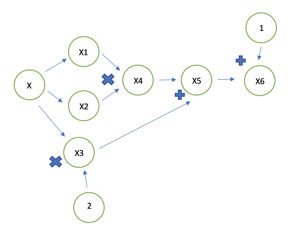
The corresponding evaluation trace looks like:

Trace	Elementary Function	Current Function value	Elementary Function Derivative	\(f(1)\)
\(x_1\)	\(x_1\)	x	1	1
\(x_2\)	\(x_2\)	x	1	1
\(x_3\)	\(x_3\)	x	1	1
\(x_4\)	\(x_1x_2\)	\(x^2\)	\(\dot{x_1}x_2 + x_1\dot{x_2}\)	2
\(x_5\)	\(x_4 + 2x_3\)	\(x^2 + 2x\)	\(\dot{x_4} + 2\dot{x_3}\)	4
\(x_6\)	\(x_5 + 1\)	\(x^2 + 2x + 1\)	\(\dot{x_5}\)	4

For the single output case, what the forward model is calculating the product of gradient and the initializaed vector p, represented mathematically as \(D_px = \Delta x \cdot p\). For the multiple output case, the forward model calculates the product of Jacobian and the initialized vector p: \(D_px = J\cdot p\). We can obtain the gradient or Jacobian matrix of the function through different seeds of the vector p.